Chapter 2 Getting to know your data
2.2 Getting data thanks to reproducibility
Last week we introduced the notion of reproducible research and said that using and publishing code (particularly if using open-source tools like R) is the way that many researchers around the world think that science ought to be done. This way of operating makes research more open, more credible, and more legitimate. It also means that we can more easily access the data used in published research. For this session, we are going to use the data from this and this paper study. In this research project, the authors tried to answer the question of whether criminal antecedents (e.g., prior convinctions) and other personal characteristics have an impact on access to employment. You can find more details about this work in episode 8 of Probable Causation, the criminology podcast.
If you want to know more about ‘Ban the Box: fair chance recruitment’ practices in the UK, you can find more information here and also can watch this short video from Leo Burnett who helped promote giving people a chance to explain their past. This could give you a better understanding of this issue.
Amanda Agan and Sonja Starr developed a randomised experiment in which they created 15,220 fake resumes randomly generating these critical characteristics (such as having a criminal record) and used these resumes to send online job applications to low-skill, entry-level job openings in New Jersey and New York City. All the fictitious applicants were male and about 21 to 22 years old. These kinds of experiments are very common among researchers who want to explore through these “audits” whether some personal characteristics are discriminated against in the labour market.
Because Amanda Agan and Sonja Starr conformed to reproducible standards when doing their research, we can access this data from the Harvard Dataverse (a repository for open research data). Click here to locate the data.
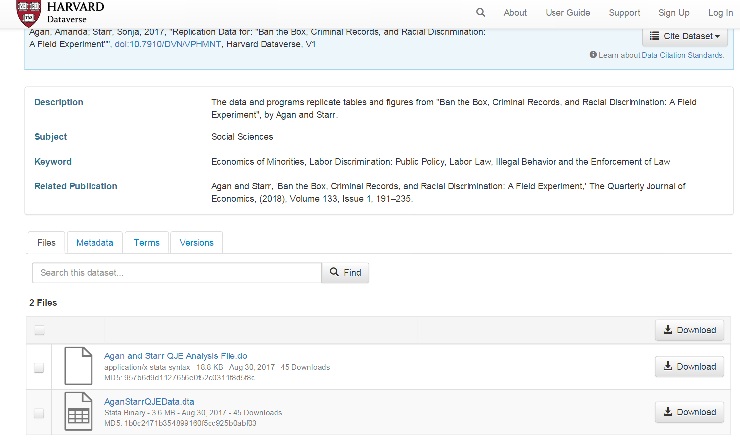
On this page, you can see a download section and some files that can be accessed. One of them contains analytic code pertaining to the study, and the other contains the data. You also see a link called metadata. Metadata is data about data – it provides you with some information about the data. If you click on metadata, you will see a reference to the software the authors used (STATA) at the bottom. So we know these files are in STATA, a proprietary format. Let’s download the data file and then read the data into R.
You could just click “download” and then place the file in your project directory. Alternatively, and preferably, you may want to use code to make your whole work more reproducible. Think of it this way: every time you click or use drop-down menus, you are doing things that others cannot reproduce because there won’t be a written record of your steps. You will need to do some clicking to find the required URL for writing your code. The file we want is the AganStarrQJEData.dta. Click on the name of this file. You will be taken to another webpage. You will see the download URL on it. Copy and paste this URL into your code below.
#First, let's import the data using an URL address:
library(haven)
banbox <- read_dta("https://dataverse.harvard.edu/api/access/datafile/3036350")

##Window users! R in Windows has some problems with HTTPS addresses;
#see below for some tips on this!
This data file is a STATA.dta file in our working directory. To read STATA files, we will need the haven package. This is a package developed to import different kinds of data files into R. If you don’t have it, you will need to install it. And then load it.
##IF THE CODE ABOVE DOES NOT WORK, USE THIS CODE.
##Window users! R in Windows have some problems with https addresses,
#in that case, try to use this code
#First, let's create an object with the link. Paste the copied address here:
urlfile <- "https://dataverse.harvard.edu/api/access/datafile/3036350"

#Now we can use the 'read_dta' and 'url' functions and import the data in the urlfile link
library(haven)
banbox <- read_dta(url(urlfile))
You will need to pay attention to the file extension to find the appropriate function to read in your file. For example, if something has the extension .sav, it is a file used by the software SPSS. To read this, for example, you would use the read_spss() function in the haven package.
Some other file types need other packages. For example, to read in comma-separated values or .csv files, you can use the read_csv() function from the readr package. To read in Excel files, you would use the appropriate function from the readxl package, which might be read_xls() or read_xlsx(), depending on the file extension.
2.3 Getting a sense of your data
2.3.1 First steps
What is the first thing you need to ask yourself when you look at a dataset? Data are often too big to look at the whole thing. It is almost always impossible to eyeball the entire dataset and see what you have in terms of interesting patterns or potential problems. It is often a case of information overload, and we want to be able to extract what is relevant and important about it. But where do you start? You can find a brief but very useful overview put together by Steph de Silva in the image below. Read it before we carry on.
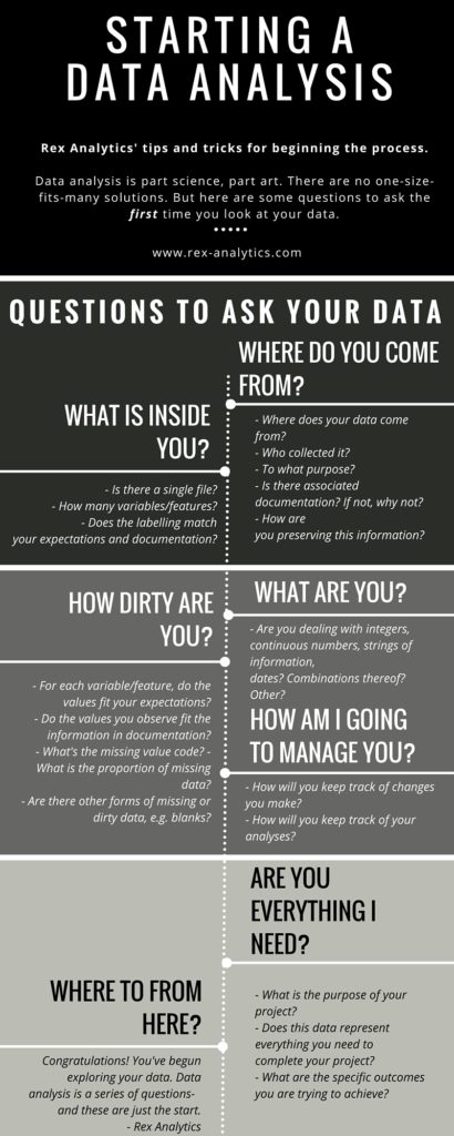
As Mara Averick suggests, this also makes for good relationship advice!

Here, we will introduce a few functions that will help you make sense of what you have just downloaded. Summarising the data is the first step in any analysis, and it is also used to find potential problems with the data. Regarding the latter, you want to look out for missing values, values outside the expected range (e.g., someone aged 200 years), values that seem to be in the wrong units, mislabeled variables, or variables that seem to be the wrong class (e.g., a quantitative variable encoded as a factor).
Let’s start with the basic things you always look at first in a dataset. You can see in the Environment window that banbox has 14813 observations (rows) of 62 variables (columns). You can also obtain this information using code. Here, you want the DIMensions of the data frame (the number of rows and columns), so you use the dim() function:
## [1] 14813 62Looking at this information will help you to diagnose whether there was any trouble getting your data into R (e.g., imagine you know there should be more cases or more variables). You may also want to have a look at the names of the columns using the names() function. We will see the names of the variables.
##  [1] "nj"                   "nyc"                  "app_date_d"
##  [4] "pre"                  "post"                 "storeid"
##  [7] "chain_id"             "center"               "crimbox"
## [10] "crime"                "drugcrime"            "propertycrime"
## [13] "ged"                  "empgap"               "white"
## [16] "black"                "remover"              "noncomplier_store"
## [19] "balanced"             "response"             "response_date_d"
## [22] "daystoresponse"       "interview"            "cogroup_comb"
## [25] "cogroup_njnyc"        "post_cogroup_njnyc"   "white_cogroup_njnyc"
## [28] "ged_cogroup_njnyc"    "empgap_cogroup_njnyc" "box_white"
## [31] "pre_white"            "post_white"           "white_nj"
## [34] "post_remover_ged"     "post_ged"             "remover_ged"
## [37] "post_remover_empgap"  "post_empgap"          "remover_empgap"
## [40] "post_remover_white"   "post_remover"         "remover_white"
## [43] "raerror"              "retail"               "num_stores"
## [46] "avg_salesvolume"      "avg_num_employees"    "retail_white"
## [49] "retail_post"          "retail_post_white"    "percblack"
## [52] "percwhite"            "tot_crime_rate"       "nocrimbox"
## [55] "nocrime_box"          "nocrime_pre"          "response_white"
## [58] "response_black"       "response_ged"         "response_hsd"
## [61] "response_empgap"      "response_noempgap"
As you may notice, these names may be hard to interpret. If you open the dataset in the data viewer of RStudio (using View), you will see that each column has a variable name and underneath a longer and more meaningful variable label that tells you what each variable means.
2.3.2 On tibbles and labelled vectors
You also want to understand what the banbox object actually is. You can do that using the class() function:
## [1] "tbl_df" "tbl" "data.frame"What does tbl stand for? It refers to tibbles. This is essentially a new type of data structure introduced into R. Tibbles are data frames, but a particular type. There are some advantages to tibbles, but honestly, they’re not that important. For now, you can just think of tibbles as data frames (and vice versa).
The R language has been around for a while, and sometimes, things that made sense a couple of decades ago make less sense now. A number of programmers are trying to create code that is more modern and more useful today. They are doing this by introducing a set of packages that speak to each other in order to modernise R without breaking existing code. You can think of it as an easier and more efficient modern dialect of R. This set of packages is called the tidyverse. Tibbles are data frames that have been optimised for use with this new set of packages. You can read a bit more about tibbles here.
You can also look at the class of each individual column. As discussed, the class of the variable lets us know, for example, if it is an integer (number), character, or factor.
To get the class of one variable, you pass it to the class() function. For example:
## [1] "haven_labelled" "vctrs_vctr" "double"## [1] "numeric"We talked about numeric vectors in week one. It is simply a collection of numbers. But what is a labelled vector? This is a new type of vector introduced by the haven package. Labelled vectors are categorical variables that have labels. Go to the Environment panel and left-click in the banbox object. This should open the data browser in the top left quadrant of RStudio.

If you look carefully, you will see that the various columns that include categorical variables only contain numbers. In many statistical environments, such as STATA or SPSS, this is a common standard. The variables have a numeric value for each observation, and each of these numeric values is associated with a label. This made sense when computer memory was an issue - for this was an efficient way of saving resources. It also made manual data input quicker. These days, it makes perhaps less sense. However, labelled vectors give you a chance to reproduce data from other statistical environments without losing any fidelity in the import process. See what happens if we try to summarise this labelled vector. We will use the table() to provide a count of observations on the various valid values of the crime variable. It is a function that obtains your frequency distribution.
##
##    0    1
## 7323 7490
So, we see that we have 7490 observations classed as 1 and 7323 classed as 2. If only we knew what those numbers represent! Well, we actually do. We will use the attributes() function to see the different “compartments” within your “box”, your object.
## $label
## [1] "Applicant has Criminal Record"
##
## $format.stata
## [1] "%9.0g"
##
## $class
## [1] "haven_labelled" "vctrs_vctr"     "double"
##
## $labels
## No Crime    Crime
##        0        1
So, this object has different compartments. The first one is called a label, and it provides a description of what the variable measures. This is what you saw in the RStudio data viewer earlier. The second compartment explains the original format. The third one identifies the class of the vector. Whereas, the final one, labels, provides the labels that allow us to identify what the meaning of 0 and 1 mean in this context.
2.3.3 Turning variables into factors and changing the labels
Last week, we said that many R functions expect factors when you have categorical data, so typically, after you import data into R you may want to coerce your labelled vectors into factors. To do that, you need to use the as_factor() function of the haven package. Let’s see how we do that.
#This code asks R to create a new column in your banbox tibble
#that is going to be called crime_f. Typically, when you alter
#variables, you can to create a new one so that the original gets
#preserved in case you do something wrong. Then we use the
#as_factor() function to explain to R that what we want to do
#is to get the original crime variable and mutate it into
#a factor, this resulting factor is what will be stored in
#the new column.
banbox$crime_f <- as_factor(banbox$crime)
You will see now that you have 63 variables in your dataset; look at the environment to check. Let’s explore the new variable we have created (you can also look for the new variable in the data browser and see how it looks different to the original crime variable):
## [1] "factor"##
## No Crime Crime
## 7323 7490## $levels
## [1] "No Crime" "Crime"
##
## $class
## [1] "factor"
##
## $label
## [1] "Applicant has Criminal Record"So far, we have looked at single columns in your data frame one at a time. But there is a way that you can apply a function to all elements of a vector (list or data frame). You can use the functions sapply(), lapply(), and mapply() . To find out more about when to use each one see here.
For example, we can use the lapply() function to look at each column and get its class. To do so, we have to pass two arguments to the lapply() function, the first is the name of the data frame to tell it what to look through, and the second is the function we want it to apply to every column of that function.
So we want to type lapply('name of dataframe', 'name of function')
Which is:
As you can see, many variables are classed as ‘labelled’. This is common with survey data. Many of the questions in social surveys measure the answers as categorical variables (e.g., these are nominal or ordinal-level measures). In fact, with this dataset there are many variables that are encoded as numeric that really aren’t. Welcome to real-world data, where things can be a bit messy and need tidying!
See, for example, the variable black:
## [1] "numeric"##
## 0 1
## 7406 7407We know that this variable measures whether someone is black or not. When people use 0 and 1 to code binary responses, typically, they use a 1 to denote a positive response, a yes. So, I think it is fair to assume that a 1 here means the respondent is black. Because this variable is of class numeric, we cannot simply use as_factor() to assign the pre-existing labels and create a new factor. In this case, we don’t have preexisting labels since this is not a labelled vector. So what can we do to tidy this variable? We’ll need to do some further work.
#We will use a slightly different function as.factor()
banbox$black_f <- as.factor(banbox$black)
#You can check that the resulting column is a factor
class(banbox$black_f)
## [1] "factor"#But if you print the frequency distribution
#you will see the data are still presented
#in relation to 0 and 1
table(banbox$black_f)##
## 0 1
## 7406 7407#You can use the levels function to see the levels of the categories in your factor
levels(banbox$black_f)## [1] "0" "1"So, all we have done is create a new column that is a factor but still refers to 0 and 1. If we assume (rightly) that 1 means black, we have 7407 black applicants. Of course, it makes sense we only get 0 and 1 here. What else could R do? This is not a labelled vector, so there is no way for R to know that 0 and 1 mean anything other than 0 and 1, which is why those are the levels is using. But now that we have the factor, we can rename those levels. We can use the following code to do just that:
#We are using the levels function to access them and change
#them to the levels we specify with the c() function. Be
#careful here because the order we specify here will map
#out to the order of the existing levels.
#So given that 1 is black and black is the second level
#(as shown when printing the results above) you want to make sure that in the c()
#you write black as the second level.
levels(banbox$black_f) <- c("non-Black", "Black")
table(banbox$black_f)
##
## non-Black Black
## 7406 7407This gives you an idea of the kind of transformations you often want to perform to make your data more useful for your purposes. But let’s keep looking at functions you can use to explore your dataset.
2.3.4 Looking for missing data and other anomalies
You can, for example, use the head() function if you just want to visualise the values for the first few cases in your dataset. The next code, for example, asks for the values for the first two cases. If you want a different number to be shown, you just need to change the number you are passing as an argument.
In the same way, you could look at the last two cases in your dataset using tail():
It is good practice to do this to ensure R has read the data correctly and there’s nothing terribly wrong with your dataset. If you have access to STATA you can open the original file in STATA and check if there are any discrepancies, for example. Glimpsing your data in this way can also give you a first impression of what the data looks like.
One thing you may also want to do is to see if there are any missing values. For that, we can use the is.na() function. Missing values in R are coded as NA. The code below, for example, asks for NA values for the variable response_black in the banbox object for observations 1 to 10:
## [1] FALSE TRUE TRUE FALSE FALSE TRUE TRUE TRUE FALSE TRUEThe result is a logical vector that tells us if it is true that there is missing (NA) data for each of those first ten observations. You can see that there are 6 observations out of those 10 that have missing values for this variable.
## [1] 7406The above is asking R to sum up how many cases are TRUE NA in this variable. When reading a logical vector like the one we are creating, R will treat the FALSE elements as 0s and the TRUE elements as 1s. So basically, the sum() function will count the number of TRUE cases returned by the is.na() function.
You can use a bit of a hack to get the proportion of missing cases instead of the count:
## [1] 0.4999662This code exploits the mathematical fact that the mean of binary outcomes (0 or 1) gives you the proportion of ones in your data. You could verify this in R using a different method, if you’d like (remember that trying stuff out, making mistakes and getting errors is just part of the process of learning R!).
As a rule of thumb, if you see more than 5% of the cases declared as NA, you need to start thinking about the implications of this. Beware of formulaic application of rules of thumb such as this, though! In this case, we know that 49%% of the observations have missing values in this variable. When you see things like this the first thing to do is to look at the codebook or documentation to try to get some clues as to why there are so many missing cases. With survey data, you often have questions that are simply not asked to everybody, so it’s not necessarily that something went very wrong with the data collection but simply that the variable in question was only used with a subset of the sample. Therefore, any analysis you do using this question will only relate to that particular subset of cases.
There is a whole field of statistics devoted to doing analysis when missing data is a problem. R has extensive capabilities for dealing with missing data -see, for example here. For the purpose of this introductory course, however, we only explain how to do analysis that ignores missing data. This is often referred to as a full/complete case analysis because you only use observations for which you have full information in all the variables you employ. You would cover techniques for dealing with this sort of issue in more advanced courses.
2.4 Data wrangling with dplyr
The data analysis workflow has a number of stages. The diagram below (produced by Hadley Wickham) is a nice illustration of this process:
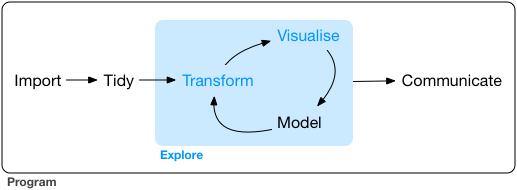
We have started to see different ways of bringing data into R. And we have also started to see how we can explore our data. It is now time we start discussing one of the following stages, transform. A good deal of time and effort, in data analysis, is devoted to this. You get your data, and then you have to transform it so that you can answer the questions you want to address in your research. We have already seen, for example, how to turn variables into factors, but there are other things you may want to do.
R offers a great deal of flexibility in how to transform your data; here, we are going to illustrate some of the functionality of the dplyr package for data carpentry (a term people use to refer to this kind of operation). This package is part of the tidyverse and it aims to provide a friendly and modern take on how to work with data frames (or tibbles) in R. It offers, as the authors of the package put it, “a flexible grammar of data manipulation”.
Dplyr aims to provide a function for each basic verb of data manipulation:
filter()to select cases based on their values.arrange()to reorder the cases.select()andrename()to select variables based on their names.mutate()andtransmute()to add new variables that are functions of existing variables.summarise()to condense multiple values to a single value.sample_n()andsample_frac()to take random samples.
In this session, we will introduce and practice some of these. But we won’t have time to cover everything. There is, however, a very nice set of vignettes for this package in the help files, so you can try to go through those if you want a greater degree of detail or more practice.
Now, let’s load the package:
## Warning: package 'dplyr' was built under R version 4.5.2##
## Attaching package: 'dplyr'## The following objects are masked from 'package:stats':
##
## filter, lag## The following objects are masked from 'package:base':
##
## intersect, setdiff, setequal, unionNotice that when you run this package you get a series of warnings in the console. It is telling us that some functions from certain packages are being “masked”. One of the things with a language like R is that sometimes packages introduce functions that have the same name as others that are already loaded into your session. When that happens, the newly loaded ones will override the previous ones. You can still use them, but you will have to refer to them explicitly. Otherwise, R will assume you are using the function most recently loaded:
#Example:
#If you use load dplyr and then invoke the *filter()* function
#R will assume you are using the filter function from dplyr
#rather than the *filter()* function that exist in the *stats*
#package, which is part of the basic installation of R. If
#after loading dplyr you want to use the filter function from
#the stats package, you will have to invoke it like this:
stats::filter()
#Notice the grammar, first you write the name of the package,
#then colon twice, and then the name of the function. Don't
#run this code. You would need to pass some valid arguments
#for this to produce meaningful results.
2.5 Using dplyr single verbs
One of the first operations you may want to carry out when working with data frames is to subset them based on the values of particular variables. Say we want to replicate the results reported by Agan and Starr in 2017. In this earlier paper, these researchers only used data from the period prior to the introduction of Ban the Box legislation and only used data from businesses that asked about criminal records in their online applications. How can we recreate this dataset?
For this kind of operation, we use the filter() function. Like all single verbs in dplyr, the first argument is the tibble (or data frame). The second and subsequent arguments refer to variables within that data frame, selecting rows where the expression is TRUE.
Ok, let’s filter out some information we are interested in from bandbox. If we look at the dataset, we can see that there is a variable called “crimbox” that identifies ‘applications that require information about criminal antecedents’ and there is a variable called “pre” that identifies ‘whether the application was sent before the legislation was introduced’. In this dataset, the value 1 is being used to denote positive responses. Therefore, if we want to create the 2017 dataset, we would start by selecting only data where the value in these two variables equals 1, as shown below.
#We will store the results of filtering the data in a new object that I am calling aer
#(short for the name of the journal in which the paper was published)

aer2017<- filter(banbox, crimbox == 1, pre == 1)
Notice that the number of cases equals the number of cases reported by the authors in their 2017 paper. That’s cool! So far, we have replicated the results.
You may have noticed in the code above that I wrote “==” instead of “=”. Logical operators in R are not written exactly the same way as in normal practice. Keep this in mind when you get error messages when running your code. Often, the source of your error may be that you are writing the logical operators the wrong way (as far as R is concerned). Look here for valid logic operators in R.
Earlier, we said that real-life data may have hundreds of variables, and only a few of them may be relevant to your analysis. For this week’s analysis, we want to select only a few variables that might be highly related to ‘Discrimination in Employment’. Say you only want “crime”, “ged” (a ged is a high school equivalence diploma rather than a proper high school diploma and is sometimes seen as inferior), “empgap” (a gap year on employment), “black_f”, “response”, and “daystoresponse” from this dataset. For this kind of operation, you use the select() function.
The syntax of this function is easy. First, we name the data frame object (“aer2017”), and then we list the variables. The order in which we list the variables within the select function will determine the order in which those columns appear in the new data frame we are creating. So, this is a handy function to use if you want to change the order of your columns for some reason. Since I am pretty confident I am not making a mistake, I will transform the original “aer2017” tibble rather than creating an entirely new object.
If you now look at the global environment, you will see that the “aer2017” tibble has reduced in size and now only has 6 columns. If you view the data, you will see the 6 variables we selected.
2.6 Using dplyr for grouped operations
So far, we have used dplyr single verbs for ungrouped operations. However, we can also use some of the functionality of dplyr to obtain answers to questions that relate to groups of cases within our data frame. Imagine that you want to know if applicants with a criminal record are less likely to receive a positive response from employers. How could you figure that one out? To answer this kind of question, we can use the group_by() function in conjunction with other dplyr functions. In particular, we are going to look at the summarise function.
First, we group the observations by criminal record in a new object, “aer2017_by_antecedent”. By using as_factor() in the call to the crime variable the results will be labelled later on (even though we are not changing the crime variable in the aer2017 data frame). Keep in mind that we are using as_factor() because the column crime is a labelled vector rather than a factor or a character vector, and we do this to aid interpretation (it is easier to
interpret labels than 0 and 1).
aer2017_by_antecedent <- group_by(aer2017, as_factor(crime))

#Then we run the summarise function to provide some useful
#summaries of the groups we are using: the number of cases
#and the mean of the response variable
results_1 <- summarise(aer2017_by_antecedent,
  count = n(),
  outcome = mean(response, na.rm = TRUE))

results_1 #auto-print the results stored in the newly created object
## # A tibble: 2 × 3
## `as_factor(crime)` count outcome
## <fct> <int> <dbl>
## 1 No Crime 1319 0.136
## 2 Crime 1336 0.0846Let’s look at the code in the summarise function above. First, we are asking R to place the results in an object we are calling “results”. Then, we specify that we want to group the data in the way we specified in our group_by() function before, that is, by criminal record. Then, we pass two arguments. Each of these arguments is creating a new variable in the resulting object called “results”. The first variable we are creating is called “count” by saying this equals “n()”, we are specifying to R that this new variable simply counts the number of cases in each of the grouping categories. The second variable we are creating is called “outcome”, and to compute this variable, we are asking R to compute the mean of the variable response for each of the two groups of applicants defined in “by_antecedents” (those with records, those without). Remember that the variable response in the “aer2017” data frame was coded as a numeric variable, even though, in truth, it is categorical in nature (there was a response, or not, from the employers). It doesn’t really matter. Taking the mean of a binary variable, in this case, is mathematically equivalent to computing a proportion, as we discussed earlier.
So, what we see here is that about 13.6% of applicants with no criminal record received a positive response from their employers, whereas only 8% of those with criminal records did receive such a response. Given that the assignation of a criminal record was randomised to the applicants, there’s a pretty good chance that no other confounders are influencing this outcome. And that is the beauty of randomised experiments. You may be in a position to make stronger claims about your results.
2.7 Making comparisons with numerical outcomes
We have been looking at relationships so far between categorical variables, specifically between having a criminal record (yes or no), race (black or white), and receiving a positive response from employers (yes or no). Often, we may be interested in looking at the impact of a factor on a numerical outcome. The researchers measured such an outcome in the banbox object. The variable “daystoresponse” tells us how long it took the employers to provide a positive response. Let’s look at this variable:
##    Min. 1st Qu.  Median    Mean 3rd Qu.    Max.    NA's
##    0.00    3.00   10.00   19.48   28.00  153.00   14361
The summary() function provides some useful stats for numerical variables. We obtain the minimum and maximum values, the 25th percentile, the median, the mean, the 75th percentile, and the number of missing data (NA). You can see the massive amount of missing data here. Most cases have missing data on this variable. Clearly, this is a function of, first and foremost, the fact that the number of days to receive a positive response will only be collected in cases where there was a positive response! However, even accounting for that, it is clear that this information is also missing in many cases that received a positive response. So, given all of this, we need to be very careful when interpreting this variable. However, because it is the only numeric variable here, we will use it to illustrate some handy functions.
We could do as before and get results by groups. Let’s look at the impact of race on days to response:
banbox_by_race <- group_by(banbox, black_f)
results_2 <- summarise(banbox_by_race,
  avg_delay = mean(daystoresponse, na.rm = TRUE))
results_2
## # A tibble: 2 × 2
## black_f avg_delay
## <fct> <dbl>
## 1 non-Black 18.7
## 2 Black 20.4We can see that the average delay seems to be longer for ‘Black’ applicants than ‘White’ applicants.
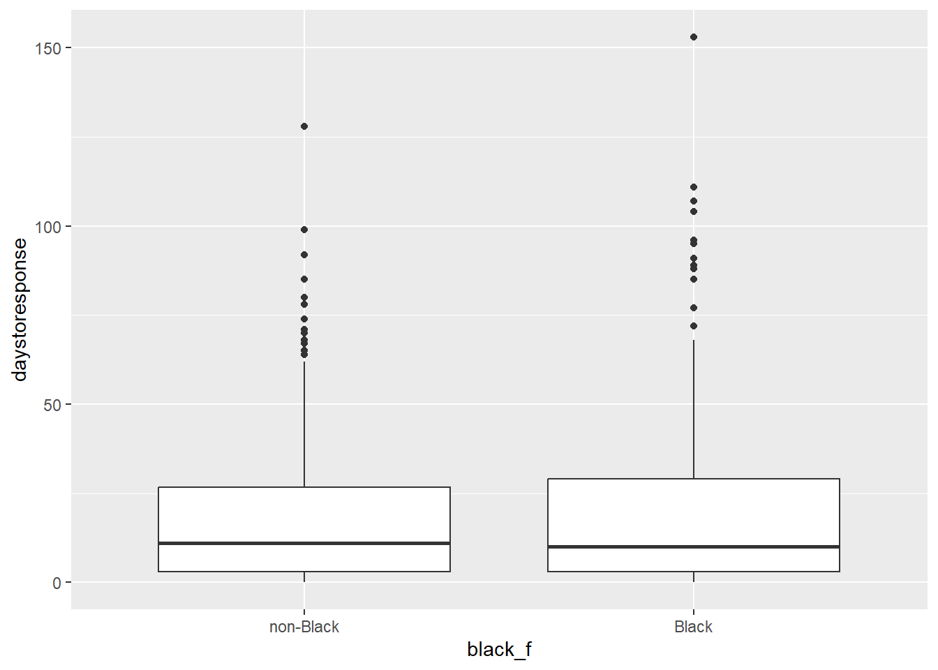
However, we could also try to represent these differences graphically. The problem with comparing groups on quantitative variables using numerical summaries, such as the mean, is that these comparisons hide more than they show. We want to see the full distribution, not just the mean. For this, we are going to use ggplot2, the main graphical package we will use this semester. We won’t get into the details of this package or what the code below means, but just try to run it. We will cover graphics in R in the next section. This is just a taster for it.
Watch this video and see if you can interpret the results portrayed here. What do you think?
Overall, the outcomes are worse for ‘Black’ applicants, and in fact, the authors find that employers substantially increase discrimination on the basis of race after ban the box goes into effect. You can now replicate these findings with the data provided. by applying the new skills you’ve learned this week!
2.8 Summary
This week, we used the following R functions:
read data: ‘haven’ package
- read_dta()
explore data
- dim()
- names()
- class()
- attribute()
- head()
- tail()
- table()
- lapply()
- sum()
- mean()
transform variables into factor variables
- as_factor()
missing variable
- is.na()
‘dplyr’ package
- filter()
- select()
- group_by()
- summarise()